Representing a tree using a list

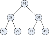
When Sorting Out Sorting got to Heapsort your first thought on seeing the tree might be "What is that thing?!"

Computer scientists call them trees — even though they look more like root systems than tree branches! We apologize, but it's all because we used to draw them on paper working down the page so as they grew we would add "branches" downward in the direction we were used to writing. There is some jargon used to describe their parts:

the circles are called nodes,
the lines are called branches,
the node at the top is called the root,
and the nodes along the bottom are called leaves.

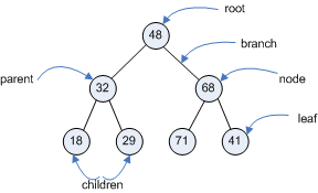
You can also see that computer scientists don't worry about mixing metaphors.

the node directly above another one is its parent (like in a family tree),
the nodes directly below a node are its children.

(There are in fact many types of trees used in Computer Science. This is a balanced binary tree. Binary because each node has at most two children, and balanced because "it's all filled in", or more formally because all paths from root to leaf have the same length.)

Your second thought as you watched the tree operations in the video might be to wonder how on earth you'd write code to work with it. We've worked with lists and strings and tuples and dictionaries, but none of them look like a tree, and at first glance none of them seem to be good candidates to represent something like a tree.

To see how we can do it let's look our list and tree together and see how we might map one onto the other.

lst = [ 48, 32, 68, 18, 29, 71, 41 ]

"Working with the tree" means being able to follow the branches to get from node to node. Notice that at any instant at most three movements are possible:

From a node down to its left child
From a node down to its right child
From a node up to its parent

To see how we might do that in the list let me draw arrows on the list to show how the values are linked in the tree:

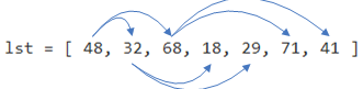
Since list operations work with the list indices let me replace the list values with their corresponding indices.

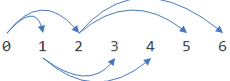
And now let's look for patterns! How about from nodes to their left children?

parent node index	0	1	2
left child index	1	3	5

Perhaps you can see the relationship here? The index of a left child is twice the index of its parent plus one. Or in Python,

def left_child(node):
    return 2*node + 1

Now, how about from nodes to their right children?

parent node index	0	1	2
right child index	2	4	6

Most students find this one less obvious, from 0 to 2 looks like we add two, from 1 to 4 looks like we multiply by four and from 2 to 6 looks like we multiply by three. No good pattern there. So look at it another way: we can see in the diagram above that the right child always comes right after the left child in the list, so its index will be exactly one greater, i.e. its index will be (2*node + 1) + 1, which is 2*node + 1 + 1 or 2*node + 2. Or in Python,

def right_child(node):
    return 2*node + 2

And finally child to parent:

child node index	0	1	2	3	4	5	6
parent index	-	0	0	1	1	2	2

This is almost a divide by two pattern which makes sense: since we got from parents to children by multiplying by two and adding, we should be able to get back by subtracting and then dividing by two:

def parent(node):
    return (node-1)/2

These three functions, left_child, right_child and parent will let us move through a list as though it were a heap. Most often we move forward through a list by incrementing an index by 1 and backward by decrementing it by 1. These functions calculate how far to move based on where we are to simulate the movement though a tree. Using them we will seem to bounce around the list by jumping back and forth, but the jumps aren't random they are carefully calibrated to replicate moving through a tree. So we can represent a Heap in a list just by modifying how we move through the list.